Housingcosts

12 Jan 2020 - Roberto Lambert

INTRODUCTION

In this project, the monthly housing cost is predicted by applying several supervised machine learning models available in the Python scikit-learn library. A potential home buyer could benefit from this machine learning application by providing the user a cost estimate of a property before closing the deal. Government agencies could use this application to identify homes in financial distress in a given region, thereby influencing their policy decisions.

DATA

The data set used is called the Housing Affordability Data System (HADS) which consists of individual datasets spanning the years 1985 to 2013. The data sets are available for download here: American Housing Survey: Housing Affordability Data System. The HADS data are sourced from the American Housing Survey (AHS) national sample microdata and the AHS metropolitan sample microdata. Therefore, more details can be obtained by referring to the AHS data. Each row in the data is an observation of a housing unit. The features fall under 4 categories:

• Cost measures: Utility costs, mortgage payments, HOA fees
• Housing unit characteristics: number of bedrooms, year built, location, structure type
• Household characteristics: income, number of people, rent/owner status
• Local market conditions: median income, fair market rent, poverty level income

To avoid data leakage issues, the features corresponding to cost measures are not fed into the machine learning models. The table below lists the features used to predict the monthly housing cost.

The HADS data files provide more features which are not included in the following analysis. These discarded variables are related to either LMED or INCRELAMIPCT.

Note that the features starting with string FMT (for formatted) are categorical variables. Therefore one-hot encoding was applied to these, ending up with with a 29-dimensional feature space. Following various data clearning/wrangling steps, the data set ends up having 486,785 observations.

For the analysis that follows, Python code was written in various Jupyter notebooks. The notebook files can be found here

MODELS

Two supervised learning algorithms are applied to predict the monthly housing cost (column name is ZSMHC in data files): ridge linear and random forest. The data is split into a test and training set. The training set is used to fit the model and the test data is used to calculate the model’s score. The table below lists the scores for the different models¹:

Ridge Linear Model

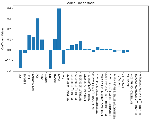
This model is applied due to its simplicity and easy interpretability of the output coefficients. At first, the hyperparameter alpha is tuned over the range from 0.01 to 100. The best value was found to be an alpha of 10. However, the score value was roughly the same across all values of alpha used (score was about 0.57). In order to compare the relative importance of the coefficients, the data was scaled to mean 0 and variance 1, and the train scaled data was fitted to a linear ridge instance with alpha set to 10. The corresponding coefficients for the scaled data are plotted below.

Random Forest

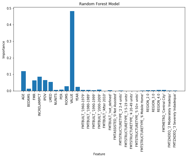
The next model used is the random forest. This is a popular model that can account for nonlinear effects in the data, unlike the ridge linear model. The training data is fed into an instance of a random forest model with default parameters. The score on the test data is around 0.61. Next the training data set is used for 3-fold cross validation, obtaining scores in the 0.60-0.62 range. The feature importance values are plotted below. The importance values add up to one. The higher a feature’s importance value, the more important that feature is.

It is to be noted that parameter tuning was performed over the following parameter grid²:

Instead of scanning the entire parameter space, 100 parameter combinations were chosen at random and the score was evaluated over these points. Over these 100 points, the score varied from 0.26 up to 0.62. The best score obtained was 0.619 with best parameter values set to:

Next, a second grid around the best parameter values listed above was created:

The score was evaluated for all the points in this grid, with scores ranging from 0.616 up to the best score of 0.619. The best score parameters turned out to be:

For the results that follow in the discussion section, n_estimators (number of trees) was set to 100 and the other parameters were set to their default values. These settings result in a score of 0.61 which is quite close to the best scores of 0.62 obtained from the parameter grid searches.

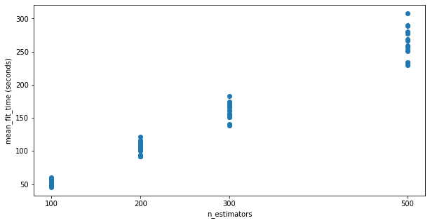
Finally, the plot below shows the average fit time versus n_estimators parameter for the points from the second grid. Note the positive linear relationship. For our purposes, a 100-tree random forest might not give the best score (although comes close), but it does run about 5 times faster than a 500-tree random forest.

Support Vector Machine

Finally, a support vector machine (SVM) model is used to predict whether or not a housing unit monthly cost is in the top 10%. For this part, a new column was created indicating whether or not a housing unit is in the top 10% of monthly housing cost for a given survey year. This column becomes the variable that the support vector machine needs to predict. The results of this model will be presented in the next section. Again the training data is used to fit the model and the test data is used to quantify the prediction accuracy.

DISCUSSION

In the table below, the top 10 features are listed for the ridge linear and random forest model. Both models agree that the housing unit market value (feature name VALUE) is the most important factor in determining the monthly housing cost.

For random forest, the second most important predicter is AGE (age of head of household), followed by INCRELAMIPCT (income). Next most important predictors for this model are variables that measure local market conditions IPOV (poverty level income), FMR (fair market rent), and LMED (median income). The least important variables include the survey year (YEAR) and variables describing the housing characteristics (ROOMS, BEDRMS, PER (number of people)).

For the linear model, the same set of variables (except for BEDRMS) are considered important; however the order of importance is different than the random forest model. Whether or not the housing unit was built in 2000-2009 was an important predictor for the linear model.

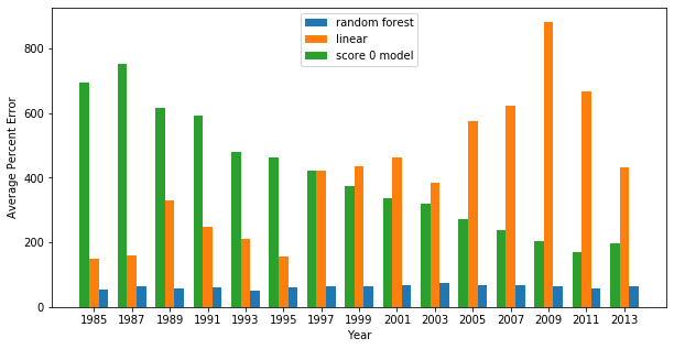
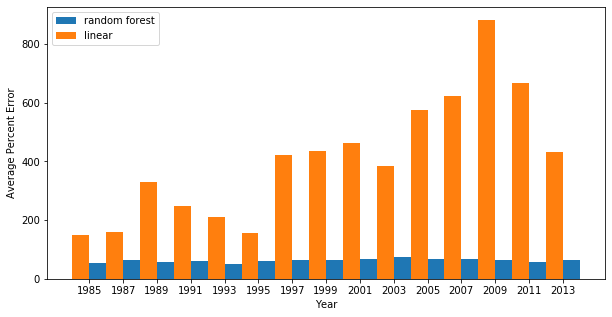
Next, the percent error is calculated for each model. As a baseline for comparison, a third model is defined which predicts the sample average, regardless of the feature values. Such a model would have a score of 0. The average percent error is plotted across survey years for linear ridge, random forest, and baseline model. The random forest has by far the smallest average percent error. For earlier survey years, the linear model performs better than the baseline model. For later survey years, the baseline model outperforms the linear model.

The plot below lists only the linear ridge and random forest models:

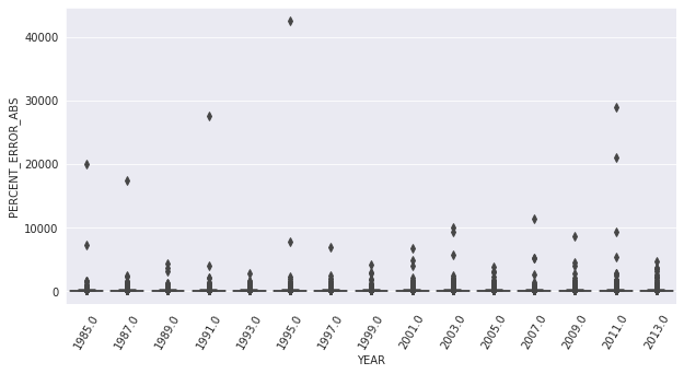
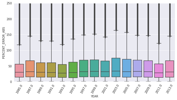
Below are boxplots of the percent error for random forest model (full plot and zommed in version):

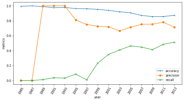
For the support vector machine, a binary variable is defined if the housing unit is above the 90th percentile for the monthly housing cost. The accuracy, precision, and recall are calculated for this variable.³ These values are listed below.

These values are plotted versus survey year below. Note that for 1985 and 1987, the second column of confusion matrix consists of zeroes. Therefore the precision is not defined and has been plotted as zero.

FURTHER WORK

To improve the predictive power of these machine learning models, the following items will be considered:

• During the data cleaning steps, a large fraction of observations had no defined VALUE column. Therefore, these rows were dropped. Instead, these missing values can be imputed based on similar entries or via by averaging over the known values.
• Consider other data sets that contain more precise location data. The current data set only specifies the 4 census regions and whether or not the housing unit is in a central city. It is well known that housing prices are higher in coastal cities and cheaper in the interior of the United States. Perhaps knowing a more precise location will help the model learn better.
• Try hyperparameter tuning/cross validation for support vector machine model.

CONCLUSION

In conclusion, a linear ridge model and random forest model were used to predict the monthly housing cost. Both models determined that the housing unit market value is an important indicator of the monthly housing cost. Both models almost had the same set of important predictor variables. However, the order of importance differed. The random forest model has on average a smaller percent error than the linear ridge model. A support vector machine is used to predict whether or not a housing unit is in the top 10% of monthly housing cost. The accuracy, precision, and recall are calculated for this model. Finally, ideas on improving the predictive power of these models are discussed.

^{1. The score function used is the r-squared value. Other score functions are available in sci-kit learn. For r-squared, a score of 1 indicates a model that exactly predicts the actual values↩}

^{2. See sci-kit learn RadomForestRegressor documentation for definition of these parameters↩}

^{3. Accuracy is the sum of true positives and true negatives divided by the total number of observations; precision is true positives divided by total predicted positive values; recall is true positives divided by total actual positive values↩}